最近在做关于深度学习项目的工作,现在记录一下本工作中了解到的,学习到的一些知识点。分有深度学习内容和 MOT 指标的内容。后面会慢慢去了解牵扯 MOT 算法层面的知识。
前向传播与反向传播?
神经网络的计算主要有两种:前向传播(foward propagation, FP)作用于没一层的输入,通过逐层计算得到输出的结果;反向传播(backward propagation, BP)作用于网络的输出,通过计算梯度由深到浅更新网络参数。
前向传播
假设上一层结点 $i,j,k,…i,j,k,…$ 等一些结点与本层的结点 $w$ 有连接,那么结点 $w$ 的值怎么算呢?就是通过上一层的 $i,j,k,…i,j,k,…$ 等结点以及对应的连接权值进行加权和运算,最终结果再加上一个偏置项(图中为了简单省略了),最后在通过一个非线性函数(即激活函数),如 ReLuReLu,sigmoidsigmoid 等函数,最后得到的结果就是本层结点 $w$ 的输出。
最终不断的通过这种方法一层层的运算,得到输出层结果。
反向传播
由于前向传播最终得到的结果,以分类为例,最终总是有误差的,那么怎么减少误差呢,当前应用广泛的一个算法就是梯度下降算法,但是求梯度就要求偏导数,下面以图中字母为例讲解一下:
设最终误差为 $E$ 且输出层的激活函数为线性激活函数,对于输出那么 $E$ 对于输出节点 $y_1$ 的偏导数是 $y_1 - t_1$ ,其中 $t_1$ 是真实值, $\frac{\partial{y_1}}{\partial{z_1}}$ 是指上面提到的激活函数, $z_1$ 是上面提到的加权和,那么这一层的 $E$ 对于 $z_1$ 的偏导数为 $\frac{\partial{E}}{\partial{z_1}}=\frac{\partial{E}}{\partial{y_1}}\frac{\partial{y_1}}{\partial{z_1}}$ 。同理,下一层也是这么计算,只不过 $\frac{\partial{E}}{\partial{y_k}}$ 计算方法变了,一直反向传播到输入层,最后有 $\frac{\partial{E}}{\partial{x_i}}=\frac{\partial{E}}{\partial{y_j}} \frac{\partial{y_j}}{\partial{z_j}}$ ,且 $\frac{\partial{z_j}}{\partial{x_i}}=w_ij$ 。然后调整这些过程中的权值,再不断进行前向传播和反向传播的过程,最终得到一个比较好的结果。
什么是模型微调fine tuning
用别人的参数、修改后的网络和自己的数据进行训练,使得参数适应自己的数据,这样一个过程,通常称之为微调 (fine tuning).
模型的微调举例说明:
我们知道,CNN 在图像识别这一领域取得了巨大的进步。如果想将 CNN 应用到我们自己的数据集上,这时通常就会面临一个问题:通常我们的 dataset 都不会特别大,一般不会超过 1 万张,甚至更少,每一类图片只有几十或者十几张。这时候,直接应用这些数据训练一个网络的想法就不可行了,因为深度学习成功的一个关键性因素就是大量带标签数据组成的训练集。如果只利用手头上这点数据,即使我们利用非常好的网络结构,也达不到很高的 performance。这时候,fine-tuning 的思想就可以很好解决我们的问题:我们通过对 ImageNet 上训练出来的模型(如CaffeNet,VGGNet,ResNet) 进行微调,然后应用到我们自己的数据集上。
微调时候网络参数是否更新?
答案:会更新。
- finetune 的过程相当于继续训练,跟直接训练的区别是初始化的时候。
- 直接训练是按照网络定义指定的方式初始化。
- finetune是用你已经有的参数文件来初始化。
fine-tuning 模型的三种状态
-
状态一:只预测,不训练。 特点:相对快、简单,针对那些已经训练好,现在要实际对未知数据进行标注的项目,非常高效;
-
状态二:训练,但只训练最后分类层。 特点:fine-tuning的模型最终的分类以及符合要求,现在只是在他们的基础上进行类别降维。
-
状态三:完全训练,分类层+之前卷积层都训练 特点:跟状态二的差异很小,当然状态三比较耗时和需要训练GPU资源,不过非常适合fine-tuning到自己想要的模型里面,预测精度相比状态二也提高不少。
多目标跟踪评估指标
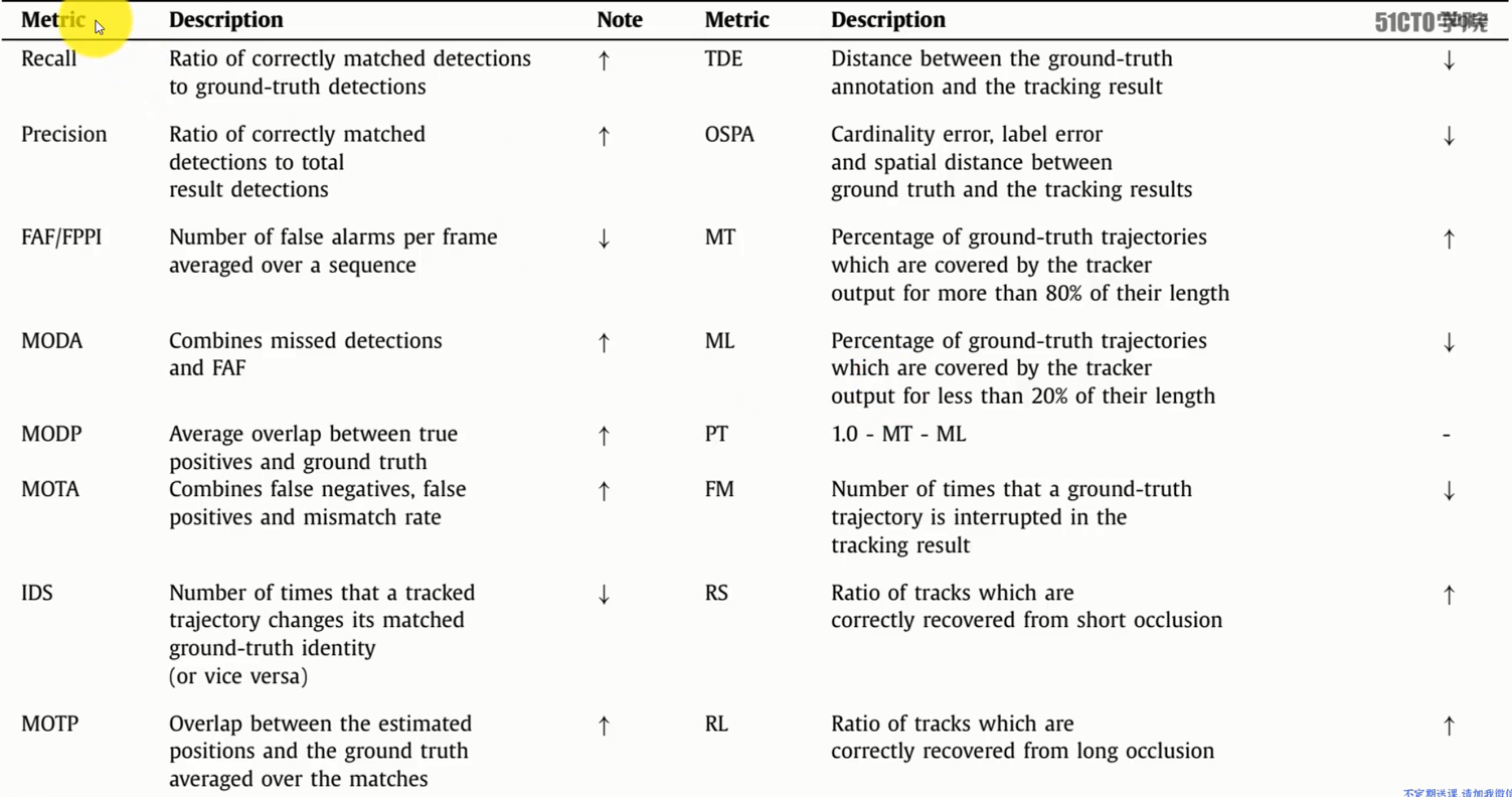
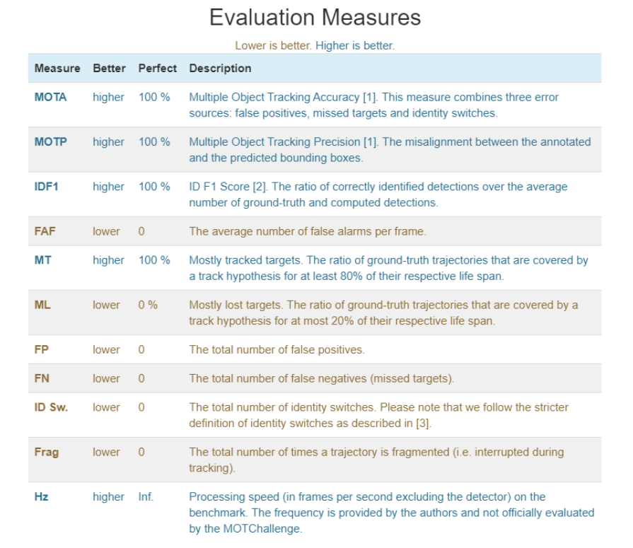
- MOTA 跟踪准确度:误报,错过目标,身份切换
- MOTP 跟踪精度:标注和预测的BBox的不匹配度
- Rcll 正确匹配的检测目标数/ground truth给出的目标数
- MT 命中的轨迹假设占ground truth 总轨迹的比例,不低于 80%
- ML 丢失的目标轨迹占 ground truth 总轨迹的比例,不超过 20%
- IDF1 正确识别的检测与平均真实数和计算检测数之比
- IDP 正确识别的计算检测的分数
- IDR 正确识别 ground truth 检测的分数
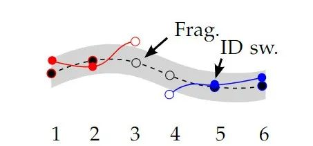
- ID_SW ID切换总数
- FP (Flase Positives) 误报总数
- FN (False Nagatives) 未命中目标的总数
- FAF 每帧的平均误报警数
- Frag 轨迹碎片化的总次数(即在跟踪过程中中断)
MOT Metrics
MOTA (Multiple Object Tracking Accuracy)
多目标跟踪精准度。衡量单个目标跟踪准确度的一个指标
MOTA summarizes three sources of errors with a single performance measure:
\[\mathrm{MOTA} = 1 - \frac{\sum_t{(\mathrm{FN}_t+\mathrm{FP}_t+\mathrm{IDSW}_t)}}{\sum_t{\mathrm{GT}_t}}\]- where $t$ is the frame index and $\mathrm{GT}$ is the number of groundtruth objects.
- $\mathrm{FN}$ are the false nagatives (漏报), i.e., the number of ground truth objects that were not detected by the method. 指 ground truth 中没有被检测到的数量。即整个视频漏报数量之和。
- $\mathrm{FP}$ are the false positives (误报), i.e., the number of objects that were falsely detected by the method but do not exist in the ground-truth. 指模型错误检测到错误的目标的数量,被检测到的目标不在 ground truth 中。即整个视频误报数量之和。
- $\mathrm{IDSW}$ is the number of identity switched, i.e., how many times a given trajectory changes from one ground-truth object to another. 值一个目标的轨迹中,从 ground truth 变到了另一个目标(id值发生改变)的次数。即整个视频误配数量之和。
We report the percentage MOTA $(-\infty, 100]$ in our benchmark. Note, that MOTA can alse be negative in cases where the number of errors made by the tracker exceeds the number of all objects in the scene.
为什么会有 $-\infty$ ,当错误的数量超过屏幕中总体目标的数量时,MOTA 则变为负
MOTA 越接近于 1 表示跟踪器性能越好,由于有跳变数的存在,当看到 MOTA 可能存在小于 0 的情况。
其中:
- 缺失率: $\frac{FN}{GT}$
- 误判率: $\frac{FP}{GT}$
- 误配率: $\frac{IDSW}{GT}$
MOTA 主要考虑的是 tracking 中所有对象匹配错误,主要是 FP、FN、IDs、MOTA 给出的是非常直观的衡量跟踪其在检测物体和保持轨迹时的性能,与目标检测精度无关。
MOTP (Multiple Object Tracking Precision)
The Multiple Object Tracking Precision is the average dissimilarity between all true positives and their corresponding ground-truth targets. For bounding box overlap, this is computed as:
\[\mathrm{MOTP} = \frac{\sum_{t,i}{d_{t,i}}}{\sum_t{c_t}}\]- where $c_t$ denotes the number of matches in frame $t$ 指在帧 $t$ 出的匹配数(匹配数是所有 true positives 和其对应的 ground-truth targets 相匹配的数量) 即第 $t$ 帧的匹配个数,对每对匹配计算匹配误差
- and $d_{t,i}$ is the bounding box overlap of target $i$ with its assigned ground-truth object in frame $t$. 指帧 $t$ 中 bounding box 和目标 ground-truth 的重叠,也就是 IOU。也相当于第 $t$ 帧下目标与其配对假设位置之间的距离
It is important to point out that MOTP is a measure of localization precision , not to be confused with the positive predictive value relevance in the context of precision / recall curves used, e.g., in object detection.
In practice, it quantifies the localization precision of the detector, and therefore, it provides little information about the actual performance of the tracker.
在目标检测中 MOTP 是对 定位精度 的度量。在实践中,它量化了检测器的定位精度,因此,它提供的关于跟踪器实际性能的信息很少。
MODA
\[\mathrm{MODA} = 1 - \frac{\sum{(\mathrm{FN}_t+\mathrm{FP}_t)}}{\sum{\mathrm{N(GT)}_t}}\]- where $\mathrm{FN}_t, \mathrm{FP}_t$ and $\mathrm{N(GT)}_t$ are represent the number of $\mathrm{FN}, \mathrm{FP}$ and $\mathrm{GT}$ , respectively, at the frame $t$. Besides,
MODP
\[\mathrm{MODP} = \frac{\sum_t\mathrm{IOU(\mathrm{GT}_t^i)}, \mathrm{D}_t^i}{\sum_t{\mathrm{M}_t}}\]- $\mathrm{IOU}(\mathrm{GT})_t^i$ is the intersection over union ( $\mathrm{IOU}$ ) of the $i$ th mapped pair between ground truth and its associated detection result, and $\mathrm{M}_t$ is the number of matches at frame $t$.
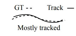
MT (Mostly Tracked)
大多数跟踪
指一条轨迹被跟踪到 80% 以上就可以认为是 MT
这里需要注意的一点是:不管这条轨迹上 ID 如何的变化(比如预测的时候发生了变化),但只要还是这条轨迹占到真实轨迹的 80% 以上就可以认为是 MT。
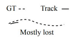
ML (Mostly Lost)
大部分缺失跟踪
指一条轨迹只被跟踪到 20% 以下就可以认为是 ML
PT (Partially Tracked)
部分跟踪。指除了 MT 、 ML ,其它的都认为是 PT
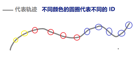
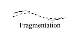
Frag / FM (Fragmentation)
就是指一条轨迹被切断的次数,按照论文的意思,应该是从跟踪到被切断计算一次 Frag,从不被跟踪到被跟踪不计算 Frag,如下图,Frag 值计算一次
ID 相关指标
The predictions-to-ground-truth mapping is established by solving a bipartite matching problem, connecting pairs with the largest temporal overlap. After the matching is established, we can compute the number of True Positive IDs (IDTP) , False Negative IDs (IDFN) , and False Positive IDs (IDFP) , that generalise the concept of per-frame TPs, FNs and FPs to tracks. Based on these quantities, we can express the Identification Precision (IDP) as:
IDP (Identification Precision)
识别精确度 (Identification Precision) 是指每个行人框中行人 ID 识别的精确度。
\[\mathrm{IDP} = \frac{\mathrm{IDTP}}{\mathrm{IDTP} + \mathrm{IDFP}}\]IDTP、IDFP 分别代表真正 ID 数和假正 ID 数,类似于混淆矩阵中的 P,只不过现在是计算 ID 的识别精确度
IDR (Identification Recall)
IDR:识别回召率 (Identification Recall) 是指每个行人框中行人 ID 识别的回召率
\[\mathrm{IDR} = \frac{\mathrm{IDTP}}{\mathrm{IDTP}+\mathrm{IDFN}}\]其中 IDFN 是假负 ID 数。
Note thar IDP and IDR are the fraction of computed (ground-truth) detections that are correctly identified.
IDF1 (Identification F-Score)
IDF1:识别 F 值 (Identification F-Score) 是指每个行人框中行人 ID 识别的 F 值
IDF1 is then expressed as a ratio of correctly identified detections over the average number of groundtruth and computed detections and balances identification precision and recall through their harmonic mean:
\[\mathrm{IDF1} = \frac{2 \cdot \mathrm{IDTP}}{2 \cdot \mathrm{IDTP} + \mathrm{IDFP} + \mathrm{IDFN}}\]