在《DEEP LEARNING IN VIDEO MULTI-OBJECT TRACKING: A SURVEY》这篇基于深度学习的多目标跟踪的综述中,描述了MOT问题中四个主要步骤:
- 给定视频原始帧。
- 运行目标检测器如 Faster R-CNN、YOLOv3、SSD 等进行检测,获取目标检测框。
- 将所有目标框中对应的目标抠出来,进行特征提取(包括表观特征或者运动特征)。
- 进行相似度计算,计算前后两帧目标之间的匹配程度(前后属于同一个目标的之间的距离比较小,不同目标的距离比较大)
- 数据关联,为每个对象分配目标的ID。
以上就是四个核心步骤,其中核心是检测,SORT论文的摘要中提到,仅仅换一个更好的检测器,就可以将目标跟踪表现提升18.9%。
DeepSORT
DeepSORT 中最大的特点是加入外观信息,借用了 ReID 领域模型来提取特征,减少了ID switch的次数。整体流程图如下:
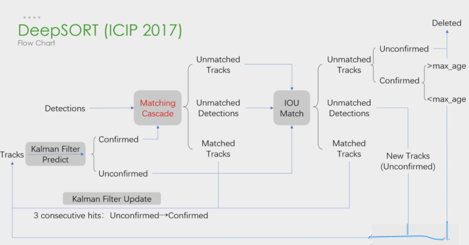
可以看出,Deep SORT算法在SORT算法的基础上增加了级联匹配(Matching Cascade)+新轨迹的确认(confirmed)。总体流程就是:
- 卡尔曼滤波器预测轨迹Tracks
- 使用匈牙利算法将预测得到的轨迹Tracks和当前帧中的detections进行匹配(级联匹配和IOU匹配)
- 卡尔曼滤波更新。
其中上图中的级联匹配展开如下:
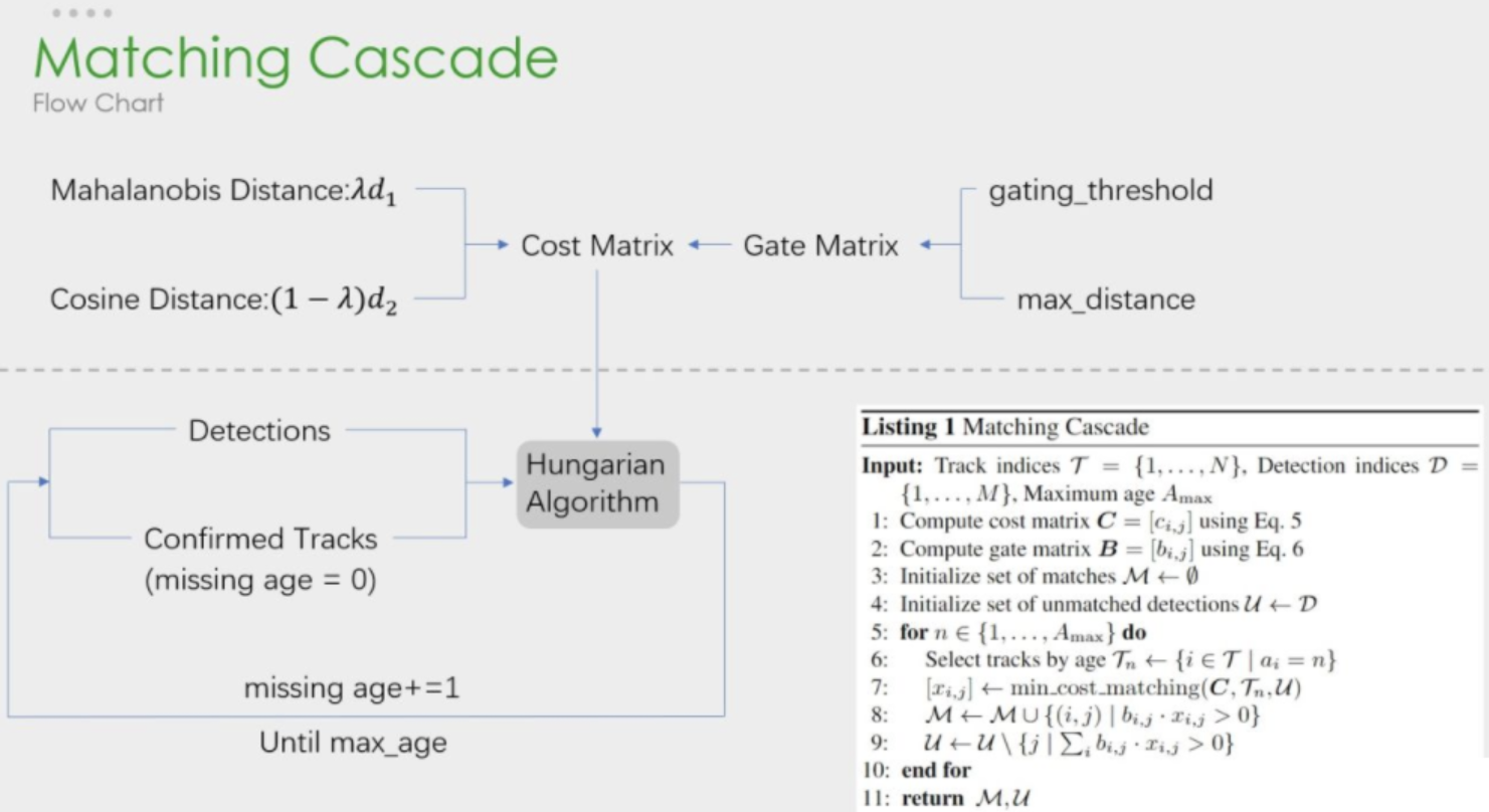
上图非常清晰地解释了如何进行级联匹配,上图由虚线划分为两部分:
上半部分中计算相似度矩阵的方法使用到了 外观模型(ReID) 和 运动模型(马氏距离) 来计算相似度,得到代价矩阵,另外一个则是门控矩阵,用于限制代价矩阵中过大的值。
下半部分中是是 级联匹配的数据关联 步骤,匹配过程是一个循环(max age个迭代,默认为70),也就是从missing age=0到missing age=70的轨迹和Detections进行匹配,没有丢失过的轨迹优先匹配,丢失较为久远的就靠后匹配。通过这部分处理,可以重新将被遮挡目标找回,降低被遮挡然后再出现的目标发生的ID Switch次数。
将 Detection 和 Track 进行匹配,所以出现几种情况
- Detection 和 Track 匹配,也就是 Matched Tracks 。普通连续跟踪的目标都属于这种情况,前后两帧都有目标,能够匹配上。
- Detection 没有找到匹配的 Track ,也就是 Unmatched Detections 。图像中突然出现新的目标的时候, Detection 无法在之前的 Track 找到匹配的目标。
- Track 没有找到匹配的 Detection ,也就是 Unmatched Tracks 。连续追踪的目标超出图像区域, Track 无法与当前任意一个 Detection 匹配。
- 以上没有涉及一种特殊的情况,就是两个目标遮挡的情况。刚刚被遮挡的目标的 Track 也无法匹配 Detection ,目标暂时从图像中消失。之后被遮挡目标再次出现的时候,应该尽量让被遮挡目标分配的ID不发生变动,减少 ID Switch 出现的次数,这就需要用到级联匹配了。
DeepSORT代码解析
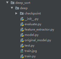
上图是 Github 库中有关 Deep SORT 的核心代码,不包括 Faster R-CNN 检测部分,所以主要将讲解这部分的几个文件
- DeepSORT 类
-
Deep ReID
- Extractor 类
- 跟踪器
- Tracker 类
- Detection 类
- NearestNerighborDistanceMetric 类
- gated_metric 类
- KalmanFilter 类
- 轨迹
- Track 类
- TrackState 类
-
DeepSort是核心类,调用其他模块,大体上可以分为三个模块:
- ReID模块,用于提取表观特征,原论文中是生成了128维的embedding。
- Track模块,轨迹类,用于保存一个Track的状态信息,是一个基本单位。
- Tracker模块,Tracker模块掌握最核心的算法,卡尔曼滤波和匈牙利算法都是通过调用这个模块来完成的。
DeepSort类对外接口非常简单:
1 | |
在外部调用的时候只需要以上两步即可,非常简单。
通过类图,对整体模块有了框架上理解,下面深入理解一下这些模块。
核心模块
Detection 类
1 | |
Detection 类用于保存通过目标检测器得到的一个检测框,包含 top left 坐标+框的宽和高,以及该 bbox 的置信度还有通过 reid 获取得到的对应的 embedding 。除此以外提供了不同 bbox 位置格式的转换方法:
- tlwh: 代表左上角坐标+宽高
- tlbr: 代表左上角坐标+右下角坐标
- xyah: 代表中心坐标+宽高比+高
Track 类
1 | |
Track类主要存储的是轨迹信息,mean和covariance是保存的框的位置和速度信息,track_id代表分配给这个轨迹的ID。state代表框的状态,有三种:
- Tentative: 不确定态,这种状态会在初始化一个Track的时候分配,并且只有在连续匹配上n_init帧才会转变为确定态。如果在处于不确定态的情况下没有匹配上任何detection,那将转变为删除态。
- Confirmed: 确定态,代表该Track确实处于匹配状态。如果当前Track属于确定态,但是失配连续达到max age次数的时候,就会被转变为删除态。
- Deleted: 删除态,说明该Track已经失效。
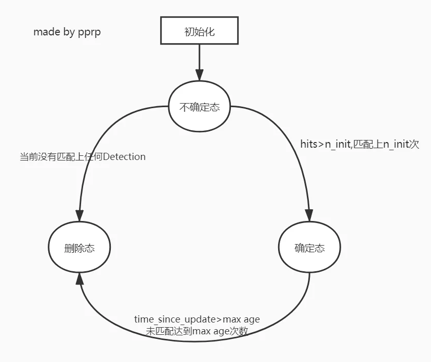
- max_age 代表一个 Track 存活期限,他需要和 time_since_update 变量进行比对。
- time_since_update 是每次轨迹调用 predict 函数的时候就会 +1,每次调用 predict 的时候就会重置为0,也就是说如果一个轨迹长时间没有 update (没有匹配上)的时候,就会不断增加,直到 time_since_update 超过 max_age (默认70),将这个 Track 从 Tracker 中的列表删除。
- hits 代表连续确认多少次,用在从不确定态转为确定态的时候。每次 Track 进行 update 的时候, hits 就会 +1, 如果 hits>n_init (默认为3),也就是连续三帧的该轨迹都得到了匹配,这时候才将不确定态转为确定态。
ReID特征提取部分
ReID 网络是独立于目标检测和跟踪器的模块,功能是提取对应 bounding box 中的 feature ,得到一个固定维度的 embedding 作为该 bbox 的代表,供计算相似度时使用。
1 | |
模型训练是按照传统 ReID 的方法进行,使用 Extractor 类的时候输入为一个 list 的图片,得到图片对应的特征。
NearestNeighborDistanceMetric类
这个类中用到了两个计算距离的函数:
- 计算欧氏距离
1 | |
- 计算余弦距离
1 | |
注意:余弦距离 = 1 - 余弦相似度。
Tracker 类
Tracker类是最核心的类,Tracker中保存了所有的轨迹信息,负责初始化第一帧的轨迹、卡尔曼滤波的预测和更新、负责级联匹配、IOU匹配等等核心工作。
1 | |
然后来看最核心的 update 函数和 match 函数,可以对照下面的流程图一起看:
update函数
1 | |
match函数
1 | |
级联匹配
下边是论文中给出的级联匹配的伪代码:
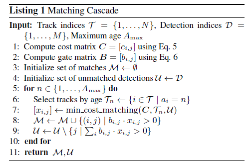
以下代码是伪代码对应的实现
1 | |
门控矩阵
门控矩阵的作用就是通过计算卡尔曼滤波的状态分布和测量值之间的距离对代价矩阵进行限制。
代价矩阵中的距离是 Track 和 Detection 之间的表观相似度,假如一个轨迹要去匹配两个表观特征非常相似的 Detection ,这样就很容易出错,但是这个时候分别让两个 Detection 计算与这个轨迹的马氏距离,并使用一个阈值 gating_threshold 进行限制,所以就可以将马氏距离较远的那个 Detection 区分开,可以降低错误的匹配。
1 | |
卡尔曼滤波器
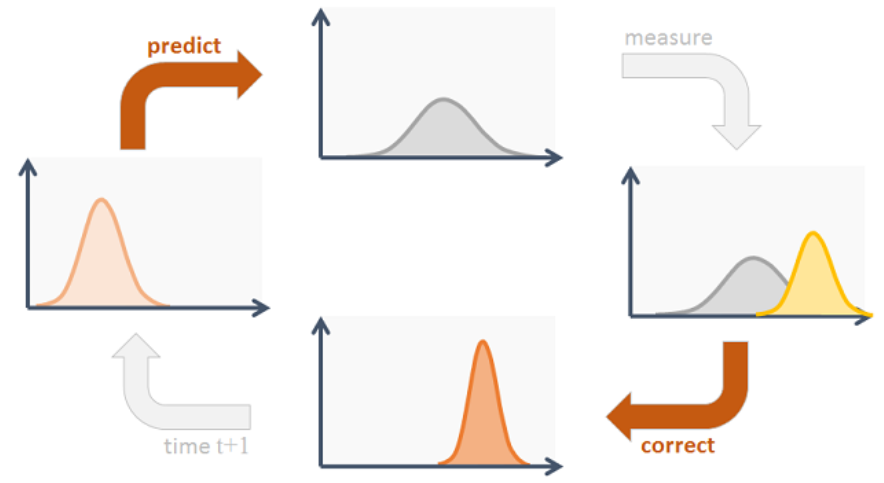
- 卡尔曼滤波首先根据当前帧(time=t)的状态进行 预测 ,得到预测下一帧的状态(time=t+1)
- 得到测量结果,在 Deep SORT 中对应的测量就是 Detection ,即目标检测器提供的检测框。
- 将预测结果和测量结果进行 更新 。
预测 分两个公式:
第一个公式:
\[{x}' = Fx\]其中 $F$ 为状态转移矩阵
第二个公式:
\[{P}' = FPF^T + Q\]$P$ 是当前帧(time=t)的协方差, $Q$ 是卡尔曼滤波器的运动估计误差,代表不确定程度。
1 | |
更新
\(y = z - H{x}'\) \(S = H{P}'H^T + R\) \(K = {P}'H^TS^{-1}\) \(x = {x}' + Ky\) \(P = (I - KH){P}'\)
1 | |
这个公式中,$z$ 是 Detection 的 mean ,不包含变化值,状态为 $[c_x,c_y,a,h]$ 。 $H$ 是测量矩阵,将 Track 的均值向量 ${x}’$ 映射到检测空间。计算的 $y$ 是 Detection 和 Track 的均值误差。
\[S = H{P}'H^T + R\]$R$ 是目标检测器的噪声矩阵,是一个 4x4 的对角矩阵。 对角线上的值分别为中心点两个坐标以及宽高的噪声。
\[K = {P}'H^TS^{-1}\]计算的是卡尔曼增益,是作用于衡量估计误差的权重。
\[x = {x}' + Ky\]更新后的均值向量 $x$ 。
\[P = (I - KH){P}'\]更新后的协方差矩阵。